Logical Modelling
You can use the following table of content to navigate around this topic:
General Information
Whereas the previous sections dealt with conceptual modeling of data warehouses, we will now have a look at the logical model of the data warehouse. Logical modeling is dependent on the type of database the data warehouse is built upon.
There are different approaches on how to store multi-dimensional data in a database. The two most important ones are ROLAP (relational OLAP) and MOLAP (multi-dimensional OLAP).
ROLAP involves a conventional relational database management system (RDBMS) that uses several flat tables to store a data cube according to the Star Schema. RDBMS-servers offer the advantage of a mature technology and a standardized query language (SQL). They are able to handle very large amounts of data at an acceptable level of performance, but a disadvantage is of course the necessity to transform the data.
MOLAP uses a specialized database server that stores the data cubes physically as a multidimensional array. This method is also referred as "pure" OLAP. Its major advantage is the faster response time due to its ability to store the data in its native form.
However this advantage vanishes with increasing amounts of data. The reason for this can be found in the sparsity of data. MDDB (Multi-Dimensional Database) servers have to fill "empty" cells in a data cube with a special N/A (not available) value, this N/A value requires the same storage capacity and machine time as a filled cell. The larger the amount of data (and empty cells) that has to be dealt with, the larger is the performance hit. Compression technique can relieve this problem to a certain extent, but a MOLAP system cannot match the performance of a ROLAP system if the amount of data gets very large.
Most of the real life implementations of Data Warehouses rely on relational databases, so in the following we will therefore concentrate on this type.
Assuming a relational database, the multi-dimensional cube model has to be mapped to flat tables. The most common approach to this task is the Star Schema and its variations. These models are based on flat tables which are denormalized to a certain extend to depict the multi-dimensional data.
Insert on Normalization
"Normalization: The process of evaluating a relation to determine whether it is in a specified normal form and, if necessary, of converting it to relations in that specified normal form." [Kroe00a]
The most common steps of normalization are shown below, the examples are taken and adapted from [Kroe00b] and [PrOs00b].
First Normal Form, 1NF
A relation is said to be in First Normal Form if each attribute of the relation is atomic, i.e. there may only be singular entries in the table.
The following table shows students having registered for various sporting activities and the fees they have to pay:
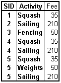
Table L.1 - First Normal Form, 1NF
Key: SID, Activity
Activity —> Fee
1NF storage anomalies:
Deletion: If student 5 stops doing weightlifting (i.e. the corresponding record is deleted), we lose the information how much this activity costs.
Update: If the fee of a certain activity changes, we have to update several entries.
Insertion: We cannot add a new activity and its corresponding fee as long as no student enlists.
Second Normal Form, 2NF
If a relation is in First Normal Form and all non-key attributes attributes depend upon the entire key, we say it is in Second Normal Form.
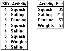
Table L.2 - Second Normal Form, 2NF
1NF storage anomalies removed:
Deletion: The record representing student 5 doing weightlifting can be deleted without losing the information about the fee of this activity.
Update: Only one record has to be modified if the fee of an activity changes.
Insertion: New activites may be added even if no students have registerd for it yet.
The students also have to pay for their rooms. The fee varies depending upon the building they live in:
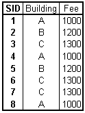
Table L.3 - Students pay for their rooms too
Key: SID
SID
Transitive dependencies among the non-key attributes!
2NF storage anomalies:
Deletion: If all students leave a certain building, the information about its fee is lost.
Update: Several records have to be updated to change the fee of a building.
Insertion: No buildings can be added without students living there.
Third Normal Form, 3NF
In order to be in Third Normal Form, a relation has to be in Second Normal Form plus there may be no transitive dependencies among the non-key attributes.
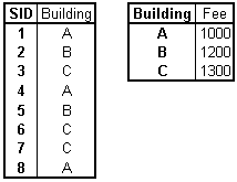
Table L.4 - Third Normal Form, 3NF
2NF storage anomalies removed:
Deletion: No information is lost if all students leave a building.
Update: If the fee of a certain building is changed, only one record has to be updated.
Insertion: There is no need for students living in a new building to add it to the database.
Students can have several majors, each major may have several professors as supervisors, but each professor supervises only one major:
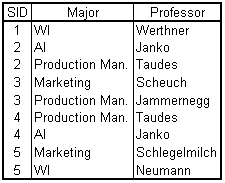
Table L.5 - Students, majors and professors
Key candidate #1: SID/Major Key candidate #2: SID/Professor Professor —> Major
Boyce-Codd Normal Form, BCNF
The Boyce-Codd Normal Form requires the relation to be in Third Normal Form. Additionally, all key candidates have to be keys.

Table L.6 - Boyce-Codd Normal Form, BCNF
Combining the students' majors and activities:
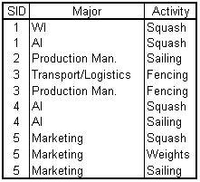
Table L.7 - The students' majors and activities
SID —> Major
SID —> Activity
Multi-value dependency!
Fourth Normal Form, 4NF
If a relation fulfills the requirements of the Boyce-Codd Normal Form and there are no multi-value dependencies, it is said to be in Forth Normal Form.
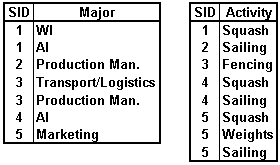
Table L.8 - Fourth Normal Form, 4NF
The Classic Star Schema
The Classic Star Schema is characterized by the use of two different kinds of tables:
a single fact table containing the key figures and a combined primary key with one element for each dimension
one or more completely denormalized dimension tables with a generated key and a level indicator that describes the hierarchical level the record belongs to
Remember the sales agent example from the Dimension Fact Modeling section (slightly simplified by the removal of the parallel hierarchy in the item-dimension): It stores the quantity sold and the returns achieved by sales agents selling certain items at a certain time. The three dimensions have the following hierarchical structure:

Table L.9 - The simplified sales agent example
This results in a Star Schema consisting of four tables:
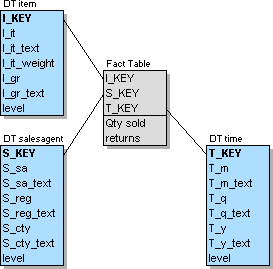
Figure L.1 - The Classic Star Schema
The link between the fact table and the three dimension tables is established by the generated keys I_KEY, S_KEY and T_KEY. Generated keys are used to ensure uniqueness and to generate the smallest possible key, allowing high performance and low maintenance.
Dimension Tables
The dimension tables contain a level field to indicate which hierarchy level the record belongs to. This is necessary to enable the storage of aggregate data. The following table shows the possible content of dimension table "item":
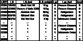
Table L.10 - Dimension table "item"
The records with the keys 00001 to 00005 represent individual items, therefore the level is 0. Records 10000 to 30000 represent item groups, entry 99999 is the highest level, the summarization of all items and item groups.
The other dimension tables may look like this:
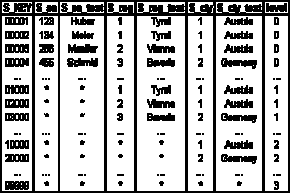
Table L.11 - Dimension table "sales agent"
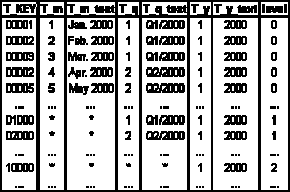
Table L.12 - Dimension table "time"
The Fact Table
The fact table is usually the largest table of the schema, it contains "the data itself", the key figures for a certain combination of item, sales agent and month. It may not only contain data at the "atomic" level, but also aggregate data for a combination like item group, country and year.
The next table shows the possible content of the fact table and an explanation for each record shown:

Table L.13 - The fact table (and an explanation of its entries)
Summary
The Classic Star Schema is a common, logical model well-suited for designing a data warehouse. The small number of tables facilitates queries and the redundant and denormalized way of storing data ensures high browsing performance. Join operations are only necessary between the single fact table and the affected dimension tables, providing high performance access. However, there are several weaknesses of the Classic Star:
First of all, when the data warehouse grows and the tables (especially the fact table) become very huge, a model designed according to the Classic Star Schema may suffer from a severe decline in performance. Today's relational database systems offer techniques like Bitmap-Indices, B-Trees, Hashing, separately kept database statistics and others to make up for the performance loss. Nevertheless the Classic Star Schema is suited primarily for small to medium amounts of data.
Another weakness is the storage of both atomic and aggregate data in the same table. This results in querying aggregate data being not faster than querying atomic data.
The Classic Star Schema with its heavily denormalized dimension tables is optimized for highest reading performance. But this comes at the cost of inflexibility. A small change in the hierarchical structure of a dimension results is many necessary updates of the according dimension table.
Another main point of criticism is the level field. There is not only the necessity to include it in every query, but it also complicates the modifications in case of a change of a hierarchical structure even further.
Extensions of the Classic Star Schema
Parallel Hierarchies
The initial sales agent example did exclude the parallel hierarchy in the item dimension for demonstration purposes. Nevertheless it is possible to create parallel hierarchies within the Star Schema. The full example's dimensions have the this hierarchical structure:

Table L.14 - The complete sales agent example
This results in the following Star Schema. The only difference is the addition of the "manufacturer" fields in the item dimension:
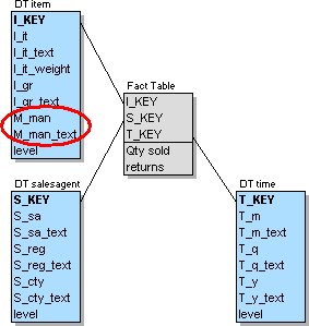
Figure L.2 - The Star Schema of the complete sales agent example
The main difference to the previous initial case is the content of the dimension tables concerned. It is necessary to replace the numeric level field by a descriptive one to distinguish the different aggregation paths at level 2 to prevent the double counting of the records. The next table shows the content of dimension table "item" including the parallel hierarchy:

Table L.15 - Dimension table "item" with a parallel hierarchy
Galaxies
Dimension tables may be reused to build another Star Schema. This is a good idea if the additional schema uses a subset of the dimensions of the first one and we wish to separate different facts of managerial interest.
Let us assume the sales agents of the initial example do not only sell goods but also attend courses to improve their skills. Further assuming that we are interested in the same granularity of data in the time dimension, we can reuse two of three dimensions of the previous example.
A nice side effect are the smaller fact tables (i.e. higher performance) compared to a "combined" solution where all the data is stored in only one schema.
The new schema stores the cost of the courses, the "course" dimension has this structure:

Table L.16 - An additional dimension for the galaxy
The galaxy containing our two stars looks like this:
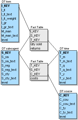
Figure L.3 - A galaxy with two stars
Improvements to the Classic Star Schema
The Fact Constellation Schema
The Fact Constellation Schema addresses the problems regarding the level field as well the performance issues with the Classic Star Schema when it comes to dealing with very large tables.
The basic idea of the Fact Constellation Schema is to split up the fact table. The records representing aggregate data are put in separate tables (aggregate fact tables - AFTs), one for each possible combination of the hierarchical levels defined in the dimension tables. This results in smaller tables and speeds up reporting on aggregate data.
The records representing atomic data are kept in the basic fact table (BFT), which is still the largest table of the set, but now considerably smaller then the fact table of a Classic Star Schema.
The number of fact tables is calculated by multiplying the number of hierarchy levels of each dimension (neglecting the total aggregation). Our example features 27 fact tables (3x3x3):
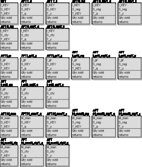
Figure L.4 - The set of fact tables
Another major improvement of the Fact Constellation Schema is that there is no need for the level attribute any more as the consolidated data is now kept in separate tables.
The Fact Constellation Schema does not change the way the dimension tables are organized. They are still in their initial denormalized form. The only difference to the Classic Star Schema is the removal of the level field:
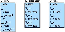
Figure L.5 - Dimension tables of the Fact Constellation Schema
As can be seen above, even the simple sales agent example results in a large set of fact tables. The necessary set of tables grows rapidly with the number of dimensions and the complexity of the dimensions' hierarchical structure.
So using of the Fact Constellation Schema means sacrificing the simplicity of the Classic Star Schema but gaining a considerable boost in performance for large data warehouses.
Partitioning and Normalization of the Dimension Tables
The Fact Constellation Schema does not change the way the dimension tables are organized, but those may also be a source of delay. Additionally they cause problems in the case of structural changes within the dimensions.
An approach called "Dimension Table Normalized by Level-Attribute" deals with these issues. Please note that the term "normalization" is not used in the sense of the normal form theory but rather means partitioning of the dimension tables by the level attribute.
This variation of the Star Schema does not change the way the facts are stored, there is still just one single fact table. Therefore the following figure only shows the dimension tables. However, due to the splitting of the dimension tables the level attribute no longer has to be maintained.
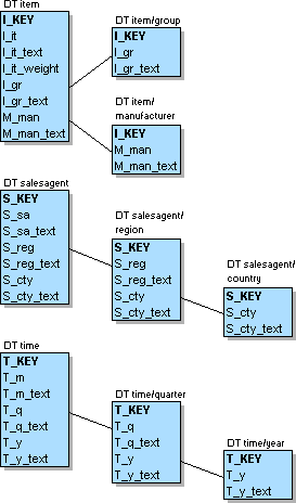
Figure L.6 - Dimension tables partitioned by the level attribute
Each dimension table includes the attributes of the higher levels, allowing aggregation within each dimension without an extra join to another table.
The content of the dimension tables belonging to the sales agent dimension is shown below, the dimension table for the highest level has been omitted, so the functionality of total aggregation has to be provided by the query:

Table L.17 - Dimension table "sales agent"

Table L.18 - Dimension table "sales agent region"

Table L.19 - Dimension table "sales agent country"
To eliminate a possible cause of inconsistency and to further increase the flexibility in case of structural changes, the dimension tables can be normalized completely. Figure L.7 shows the result:
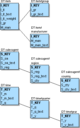
Figure L.7 - Dimension tables normalized completely
This arrangement facilitates updates within the dimension tables, reduces the storage capacity needed and allows for smaller tables. However, normalizing the dimension tables is not undisputed. The normalization comes hand in hand with a lower query performance due to the increased number of joins necessary. Ralph Kimball for example denies any advantage of normalization and advises the designer of a data warehouse to forego it completely. [Kimb96]
The Snowflake Schema
The Snowflake Schema is a combination of the Fact Constellation Schema and the "dimension table normalized by level-attribute"-approach. The fact table is split into several tables (see Figure L.4), the dimension tables are partitioned or normalized (see Figure L.6 and L.7). For the basic fact table of the sales agent example the Snowflake Schema looks like this (the dimension tables have been normalized completely):
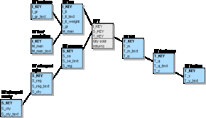
Figure L.8 - The Snowflake Schema for the basic fact table
This variation of the Classic Star Schema incorporates the advantages and disadvantages of the previously shown methods:
Structural changes in the dimensions can easily be performed
Low storage needs as compared to the Classic Star
Better performance due to smaller tables, can handle large amounts of data
Separation of atomic and aggregated data
No need for a level attribute
Rather complex, large number of tables
May cause poor browsing performance because of the normalized dimension tables ("Resist the urge to snowflake" [Kimb96])
