Aggregation Path Array
You can use the following table of content to navigate around this topic:
General Information
The Aggregation Path Array by A. Prosser and M. Ossimitz concentrates primarily on the matter of aggregate data and the decision whether aggregates should be stored (materialized) in the data warehouse. [PrOs00A] and [PrOs01]
It is often impossible to store the base cube, i.e. data at its finest level of aggregation, because the sheer amount of data cannot be handled at all or at least not at an acceptable level of performance.
Real implementations of data warehouses use pre-built aggregates (sub-cubes derived from the base cube that contain less data because of a higher aggregation level). Those sub-cubes are chosen from the set of possible derivatives based upon the end-user's requirements and access patterns. Whether a sub-cube a user is interested in is materialized or not also depends upon the effort necessary to derive it from a cube already materialized.
To communicate with the end-user the data warehouse designer needs a tool to depict the whole set of possible derivatives and their mutual dependencies. This is where the Aggregation Path Array (APA) can be used as a design tool.
Description of the Model
The APA is an array showing all sub-cubes that can be derived from the base cube. It includes a certain amount of redundancy, i.e. some of the derivative cubes may be found twice or even more often, however the redundancy-free set of sub-cubes is tagged by the algorithm used to build the APA. It is worth mentioning that the base cube itself is NOT displayed in the array.
To build the APA a definition of the dimensions is needed. Let us assume the following example: A 4-dimensional cube stores data (e.g. quantity delivered, incurred costs, …) about materials delivered by a certain supplier to a certain plant at a certain time, the dimensions have the following hierarchical structure:

Table A.1 - The dimensional structure of the introductory example
The asterisk means summarization over all elements along the corresponding dimension, it is always the highest level of aggregation.
Our example has four dimensions (n=4) and we consecutively number the aggregation levels of each dimension starting with zero. The number of the highest level of a dimension r (= the number of aggregation steps in this dimension) is referred to as i(r) (e.g. for the material dimension: i(3)=3).
The model depicts data cubes as vectors with n elements with each element representing an aggregation level of a dimension: Some examples...
The base cube (that is NOT part of the APA) is represented by the vector
v = (P_pl, S_sup, M_mat, T_w)
The sub-cube containing data about deliveries of certain materials (M_mat) to all plants (P_*) by certain supplier groups (S_gr) in certain quarters (T_q) is represented by the vector
v = (P_*, S_gr, M_mat, T_q)
The highest level of aggregation along all dimensions is displayed as
v = (P_*, S_*, M_*, T_*)
Each line of the APA shows an aggregation path from the base cube to the highest level of aggregation, so the last cell within a line is always v = (P_*, S_*, M_*, T_*). Because the base cube itself is not shown in the APA, the first cell of a line is always a vector with one dimension aggregated to level 1, e.g.
v = (P_*, S_sup, M_mat, T_w) or v = (P_pl, S_gr, M_mat, T_w)
Before building the APA we will calculate its size by using the following formulas:
The number of columns is quite obvious, it is the sum of the number of aggregation steps in all dimensions:

The number of lines of the APA is calculated by multiplying the number of aggregation steps +1 of all dimensions but the last one:

For our example this results in an array with 24 lines (L=2x3x4=24) and 10 columns (C=1+2+3+4=10).
Because of the way the number of lines of the APA is defined, it is helpful to sort the dimensions according to their number of aggregation steps to keep the APA small and the amount of redundancy low. This has already been done in our example.
The size of the redundancy-free set (including the base cube) can be calculated in the following way:

In our example the redundancy-free set consists of 120 cubes (2x3x4x5=120)
Building the Aggregation Path Array
Each cell of the APA represents a vector, but to keep the array manageable a cell only shows the dimension that has been incremented at that particular stage of the aggregation path. How to derive the underlying vector is shown below after building the APA.
The APA is built using the following algorithm: (Using a spreadsheet program like Microsoft Excel® can quite simplify this task)
Build the first line: Aggregate all dimensions to their highest level, omitting the lowest level. The dimension with the most hierarchy levels (T) should be the last. Tag all cells as part of the redundancy-free set (as they appear for the first time).

Figure A.1 - The first line of the APA
Figure A.2 shows some of the vectors represented by the cells of line 1. As stated before each cell only shows one element of the underlying vector. The other elements can be derived by inserting the highest aggregation level in each dimension found in the path to the left of a certain cell. If no entry is found, the corresponding dimension has not been aggregated yet and the lowest aggregation level is inserted.

Figure A.2 - The underlying vectors
After having built the first line, shift the last dimension n (T) through dimension n-1 (M) (to shift means to copy the line above and move the whole last dimension one step to the left in each line, inserting the cell in front of the last dimension behind it).
Highlight the cells belonging to the last dimension (T) as part of the redundancy-free set.
In our example this step results in three new lines because the penultimate dimension (M) has three aggregation steps:

Figure A.3 - The last dimension (T) is shifted through the penultimate one (M)
Shift the last two dimensions (M and T) as a block through dimension n-2 (S)
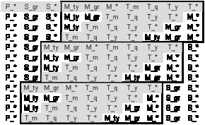
Figure A.4 - Dimensions M and T move through dimension S
Repeat this step for the remaining dimensions. In our case this means to shift dimensions n (T), n-1 (M), n-2 (S) as a block through dimension 1 (P):
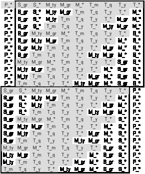
Figure A.5 - Dimensions M, T and S are shifted through dimension P
The above algorithm creates the following APA. The underlying vectors of some cells are shown for demonstration purposes:
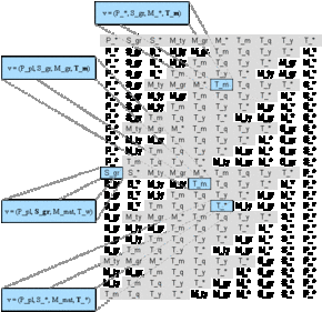
Figure A.6 - The complete APA with the redundancy-free set of cubes
Deciding which Cubes to Materialize
In the next step the end-users have to indicate which cubes they are actually interested in. They will usually not just choose individual cubes but rather whole aggregation paths. These paths have to be highlighted in the APA.
We will assume the following end-user requirements (they are highlighted in Figure A.7):
"a monthly and quarterly report for each material type, independent of the supplier and the plant" (1st blue area)
"a complete drill-down by the time dimension down to months for each supplier on a material type and group level, irrespective of the plant the goods are delivered to." (2nd blue area)
"the same drill-down by the time dimension as above for each plant on a material type and group level, independent of the supplier" (3rd blue area)
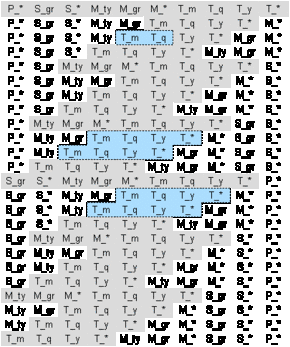
Figure A.7 - End-user requirements shown in the APA
After having depicted the cubes the end-user is interested in, an important question arises: Which cubes should actually be materialized so that all interesting cubes are derivable from the materialized ones?
If we materialize v = (P_*, S_*, M_ty, T_m), represented by the leftmost cell in the first blue area (end-user requirement 1), we will have to find out which other cubes can be derived from it.
This can be accomplished by using the following simple algorithm:
| For each line in the APA check all cells starting with the rightmost one until you find a cell that contains an element of vector v. This cell and all the ones to the right of it represent cubes derivable from v. Tag them and switch to the next line. |
The next table shows our APA after the algorithm has been applied to all lines, all cells to the right of the bold line are derivatives of v = (P_*, S_*, M_ty, T_m):
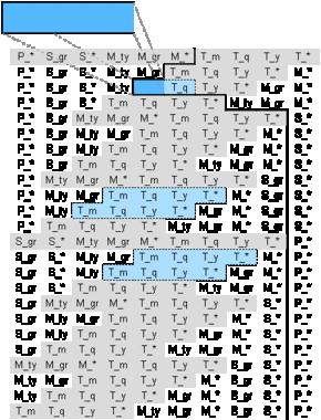
Figure A.8 - Derivatives of v = (P_*, S_*, M_ty, T_m)
As can be seen above, none of the other end-user requirements is covered by the derivatives of v = (P_*, S_*, M_ty, T_m). Therefore additional cubes have to be materialized.
Materializing cube u = (P_*, S_sup, M_ty, T_m) (leftmost cell in the second blue area representing end-user requirement 2) and cube w = (P_pl, S_*, M_ty, T_m) (leftmost cell in the third blue area representing end-user requirement 3) offers us the following sets of derivatives:
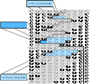
Figure A.9 - Derivatives of u = (P_*, S_sup, M_ty, T_m)
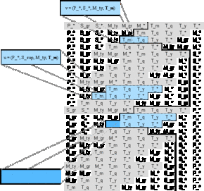
Figure A.10 - Derivatives of w = (P_pl, S_*, M_ty, T_m)
Figures A.9 and A.10 show that end-user requirement 1 is covered by both the derivatives of u and w. Considering that v = (P_*, S_*, M_ty, T_m) can easily be derived from u = (P_*, S_sup, M_ty, T_m) or w = (P_pl, S_*, M_ty, T_m) by aggregation along only one dimension simplifies the materialization decision:
| To meet the all end-user requirements, we will have to materialize the cubes u and w. Materializing cube v is probably unnecessary even from a performance point of view. |
Summary
The Aggregation Path Array offers an easy method to depict a data cube and all of its derivatives, thereby providing data warehouse designers with a tool to specify the end-user's requirements in a more formal way. The possibility to display the derivatives of a certain sub-cube simplifies materialization decisions and can also be used to plan updates of the data warehouse.
Future extensions of the APA are planned to offer support for cost functions to further optimize the materialization decisions (what are the costs of the materialization of a certain cube and what utility is gained by doing so?). The final goal of the APA's developers is the implementation of a software tool capable of creating the APA and deriving the optimal set of materialized views.
A java applet for creation and administration of the APA is already available at the courses section [Pros01]
